
Session-based Recommender Systems
FF19 · ©2021 Cloudera, Inc. All rights reserved
This is an applied research report by Cloudera Fast Forward. We write reports about emerging technologies, and conduct experiments to explore what’s possible. Read our full report on Session-based Recommender Systems below, or download the PDF, and be sure to check out our github repo for the Experiments section.
Being able to recommend an item of interest to a user (based on their past preferences) is a highly relevant problem in practice. A key trend over the past few years has been session-based recommendation algorithms that provide recommendations solely based on a user’s interactions in an ongoing session, and which do not require the existence of user profiles or their entire historical preferences. This report explores a simple, yet powerful, NLP-based approach (word2vec) to recommend a next item to a user. While NLP-based approaches are generally employed for linguistic tasks, here we exploit them to learn the structure induced by a user’s behavior or an item’s nature.
Introduction
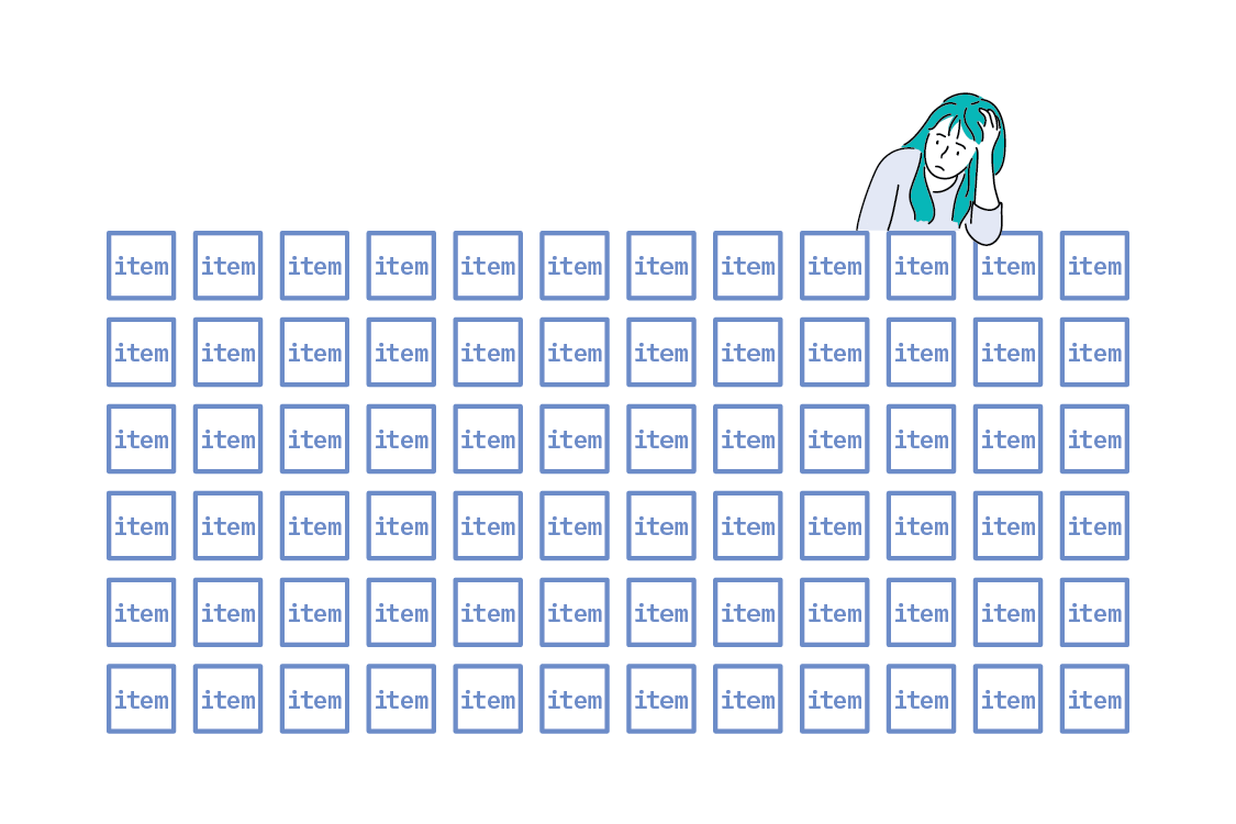
Recommendation systems have become a cornerstone of modern life, spanning sectors that include online retail, music and video streaming, and even content publishing. These systems help us navigate the sheer volume of content on the internet, allowing us to discover what’s interesting or important to us. When implemented correctly, recommendation systems help us navigate efficiently and make more informed decisions.
While this report is not comprehensive, we will touch on a variety of approaches to recommendation systems, and dig deep into one approach in particular. We’ll demonstrate how we used that approach to build a recommendation system from the ground up for an e-commerce use case, and showcase our experimental findings. Finally, we’ll also talk about many of the considerations necessary to building thoughtful, information-driven recommendation systems.
Session-based Recommender Systems
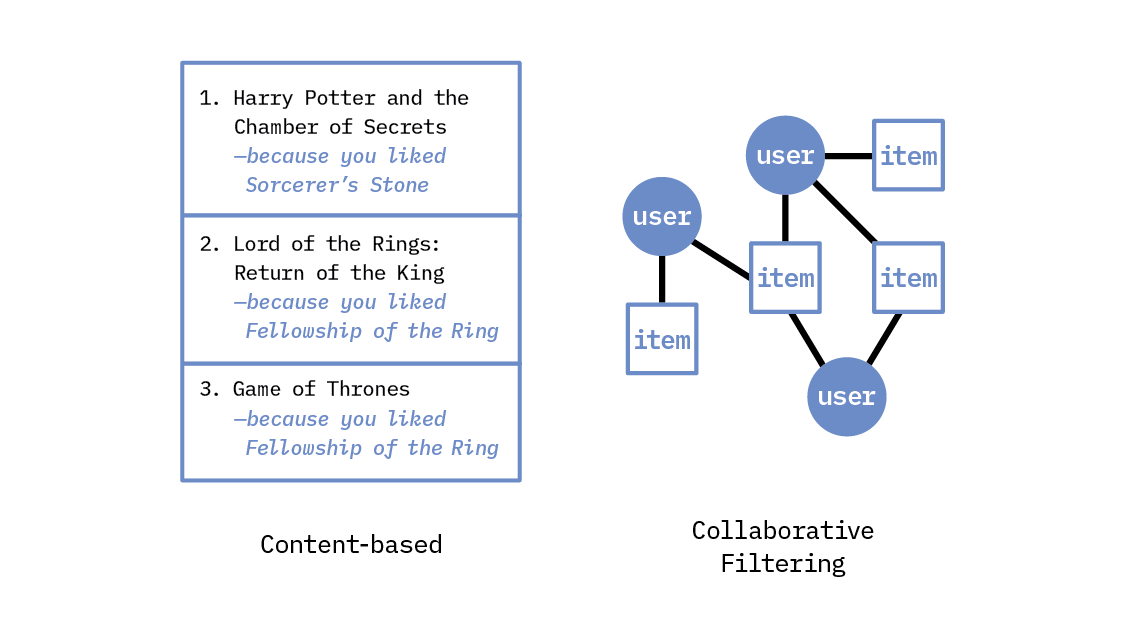
Recommendation systems are not new, and they have already achieved great success over the past ten years through a variety of approaches. These classic recommendation systems can be broadly categorized as content-based, as collaborative filtering-based, or as hybrid approaches that combine aspects of the two.
At a high level, content-based filtering makes recommendations based on user preferences for product features, as identified through either the user’s previous actions or explicit feedback. Collaborative filtering, on the other hand, utilizes user-item interactions across a population of users in order to make recommendations for one particular user, based on the preferences of other, very similar users (where similar users are identified by the items they have liked, read, bought, watched, etc.). These systems generally tend to utilize historical user-item interactions (i.e., the items that a user has clicked on in the past) to learn a user’s long-term preferences.
The underlying assumption in both of these systems is that all of the historical interactions are equally important to the user’s current preference—but in reality, this may not be true. A user’s choice of items not only depends on long-term historical preference, but also on short-term and more recent preferences.
Choices almost always have time-sensitive context; for instance, “recently viewed” or “recently purchased” items may actually be more relevant than others. These short-term preferences are embedded in the user’s most recent interactions, but may account for only a small proportion of historical interactions. In addition, a user’s preference towards certain items can tend to be dynamic rather than static; it often evolves over time.
These considerations have prompted the exploration and development of a new class of recommendation algorithms: known as session-based recommendation algorithms, these rely heavily on the user’s most recent interactions, rather than on the user’s historical preferences. In addition, this approach is especially advantageous because a user could appear anonymously—that is, a user may not be logged in or may be browsing incognito.
Why now?
While nearly unknown as of just a few years ago, session-based recommenders have grown quickly in popularity, and for several reasons. First, this method can be implemented even in the absence of historical user data, and doesn’t explicitly rely on user population statistics. This is helpful because, as just noted above, users aren’t always logged in when they browse a website, which makes session-based recommenders highly relevant.[1]
Second, a wealth of new, publicly available, session-centric datasets have been released, especially in the e-commerce domain, allowing for model development and research in this area.
Third, session-based recommenders have benefited from the rise of deep learning approaches expressly suited for sequences (more on this in Modeling Session-based Recommenders, below).
Defining the Session-based Recommender Problem Space
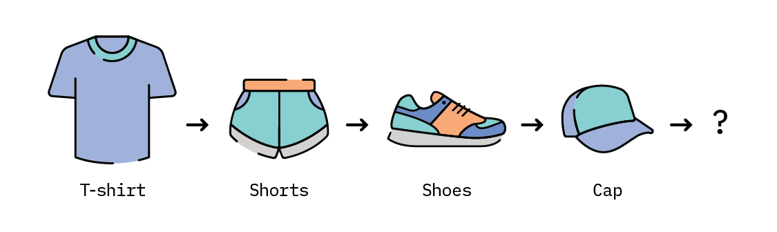
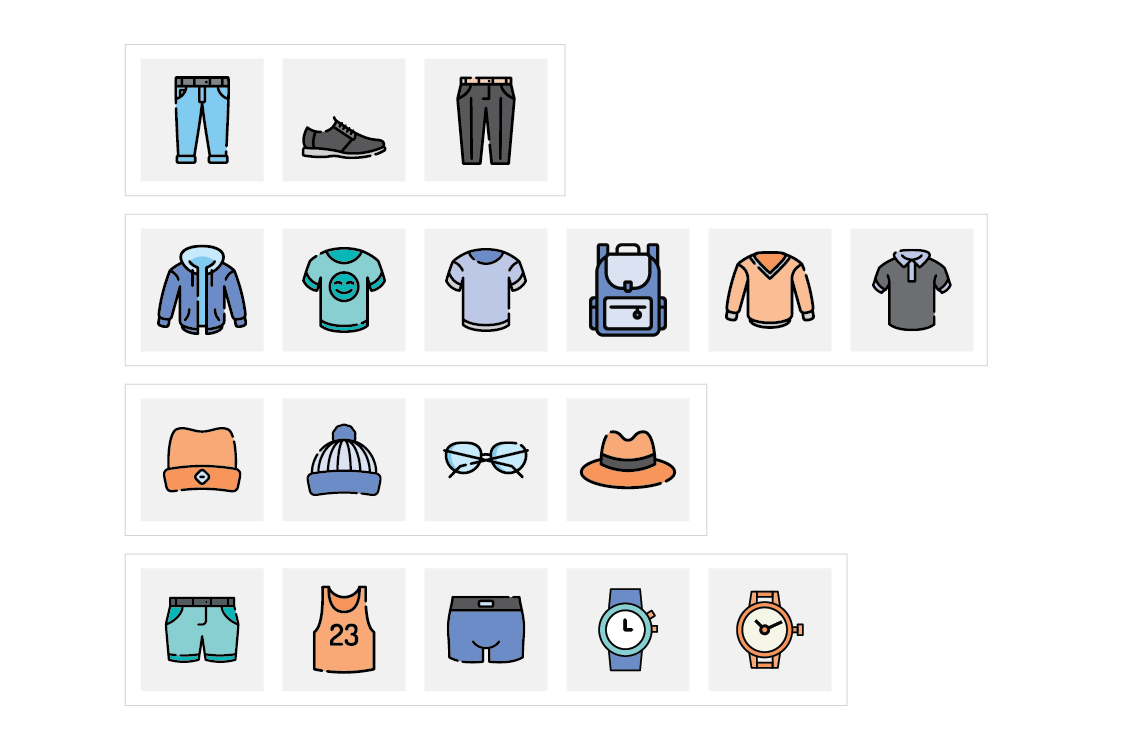
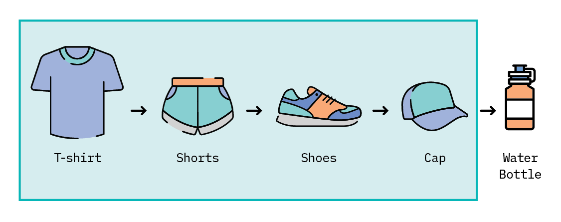
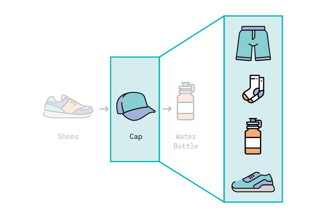
Let’s say we own a popular online shopping website for workout accessories. Rhonda, a new customer, has been browsing tops, shoes, and weights. Her browsing history looks like this:
What should we recommend to her next? Good recommendations increase the likelihood that Rhonda will see something she likes, click on it, and make a purchase. Poor recommendations will, at best, lead to no new revenue, but-even worse-could give her a negative customer experience. (You know this feeling: when a website keeps recommending something to you that you have already bought, or something that you’ve never really wanted, your impression of that website diminishes!)
We’ll consider Rhonda’s recent browsing history as a “session.” Formally, a session is composed of multiple user interactions that happen together in a continuous period of time—for instance, products purchased in a single transaction. Sessions can occur on the same day, or across several days, weeks, or months.
Our goal is to predict the product within Rhonda’s session that she will like enough to click on. This task is called next event prediction (NEP): given a series of events (Rhonda’s browsing history), we want to predict the next event (Rhonda clicking on a product we recommend to her).
In reality, this means that our model might generate a handful of recommendations based on Rhonda’s browsing history; we want to maximize the likelihood that Rhonda clicks on at least one of them. To train a model for this task, we’ll need to use historical browsing sessions from our other existing users to identify trends between products that will help us learn recommendations.
Use Cases
This problem is well-aligned with emerging real-world use cases, in which modeling short-term preferences is highly desirable. Consider the following examples in music, rental, and product spaces.[2]
Music recommendations
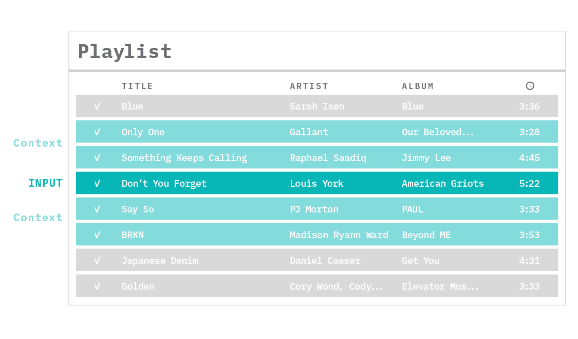
Recommending additional content that a user might like while they browse through a list of songs can change a user’s experience on a content platform.
The user’s listening queue follows a sequence. For each song the user has listened to in the past, we would want to identify the songs listened to directly before and after it, and use them to teach the machine learning model that those songs somehow belong to the same context. This allows us to find songs that are similar, and provide better recommendations.[3]
Rental recommendations
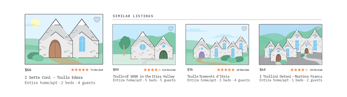
Another powerful and useful application of session-based recommendation systems occurs in any type of online marketplace. For instance, imagine a website that contains millions of diverse rental listings, and a guest exploring them in search of a place to rent for a vacation.[4] The machine learning model in such a situation should be able to leverage what the guest views during an ongoing search, and learn from these search sessions the similarities between the listings. The similarities learned by the model could potentially encode listing features-like location, price, amenities, design taste, and architecture.
Product recommendations
Leveraging emails in the forms of promotions and purchase receipts to recommend the next item to be purchased has also proven to be a strong purchase intent signal.[5] Again, the idea here is to learn a representation of products from historical sequences of product purchases, under the assumption that products with similar contexts (that is, surrounding purchases) can help recommend more meaningful and diverse suggestions for the next product a user might want to purchase.

With these examples in mind, let’s dig deeper into what it takes to design and build a session-based recommendation system for product recommendations, in the context of an online retail website.
Modeling Session-based Recommenders
There are many baselines for the next event prediction (NEP) task. The simplest and most common are designed to recommend the item that most frequently co-occurs with the last item in the session. Known as “Association Rules,”[6] this heuristic is straightforward, but doesn’t capture the complexity of the user’s session history.
More recently, deep learning approaches have begun to make waves. Variations of graph neural networks[7] and recurrent neural networks[8] have been applied to the problem with promising results, and currently represent the state of the art in NEP for several use cases. However, while these algorithms capture complexity, they can also be difficult to understand, unintuitive in their recommendations, and not always better than comparably simple algorithms (in terms of prediction accuracy).
There is still another option, though, that sits between simple heuristics and deep learning algorithms. It’s a model that can capture semantic complexity with only a single layer: word2vec.
Treating it as a NLP problem
Word2vec? Isn’t that the algorithm that made word embeddings commonplace? Yes! Word2vec uses the co-occurrence of words in a sentence to learn embeddings for each word that capture the semantic meaning of that word. At its core, word2vec is a simple, shallow neural network, with a single hidden layer. In its skip-gram version, it takes as input a word, and tries to predict the context of words around it as the output. For instance, consider this sentence:
“The cat jumped over the puddle.”[9]
Given the central word “jumped,” the model will be able to predict the surrounding words: “The,” “cat,” “over,” “the,” “puddle.”
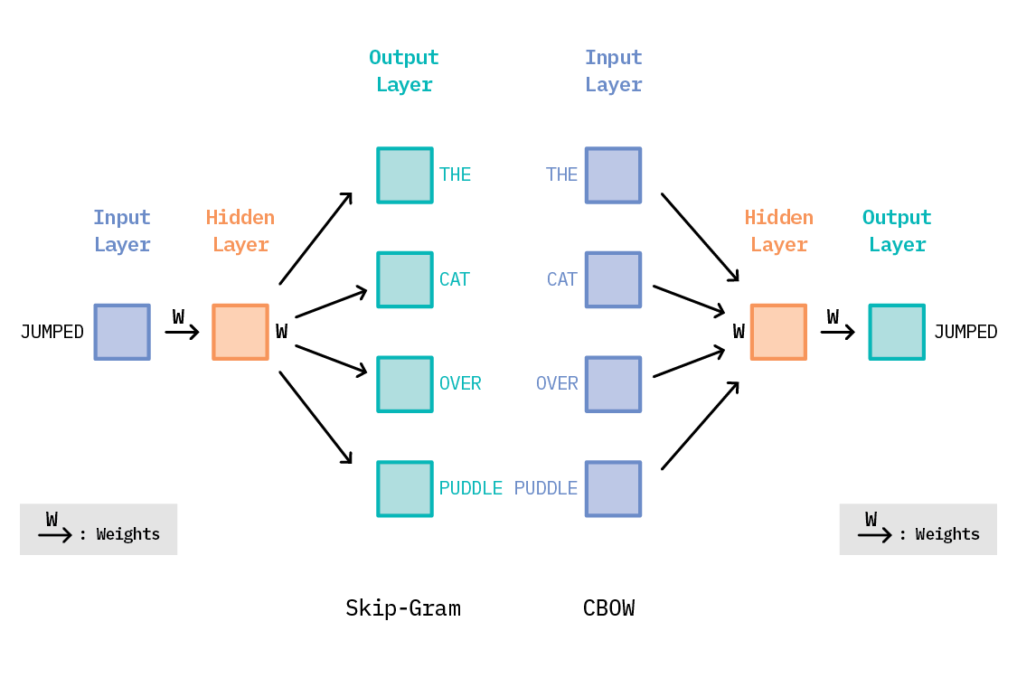
Another approach—Continuous Bag of Words (CBOW)—treats the words “The,” “cat,” “over,” “the,” and “puddle” as the context, and predicts the center word: “jumped.” For the rest of this report, we will restrict ourselves to the skip-gram model. The Ws in the above diagram represent the weight matrices that control the weight of the successive transformations we apply to the input to get the output. Training this shallow network means learning the values of these weight matrices, which gives us the output that is closest to the training data. Once trained, the output layer is usually discarded, and the hidden layer (also known as the embeddings) is used for downstream processes. These embeddings are nothing but vector representations of each word, such that similar words have vector representations that are close together in the embedding space.
How can we use this for NEP?
Let’s take another look at Rhonda’s browsing history. We can treat each session as a sentence, with each item or product in the session representing a “word.” A website’s collection of user browser histories (including Rhonda’s) will act as the corpus. Word2vec will crunch over the entire corpus, learning relationships between products in the context of user browsing behavior. The result will be a collection of embeddings: one for each product. The idea is that these learned product embeddings will contain more information than a simple heuristic, and training the word2vec algorithm is typically faster and easier than training more complex, data-hungry deep learning algorithms.
In fact, word2vec can be invoked as a reasonable approach any time we’re faced with a problem that is sequential in nature, and where the order of the sequences contains information. In this case, casting sessions as an NLP problem makes sense because we do have sequential data (user browser histories are typically ordered by time) and the order likely does matter (capturing the user’s interests as they navigate various products). While the basic algorithm can conceptually be applied to other domains, only recently has research explored this explicitly for the NEP task.[10] [11]
Evaluating Session-based Recommenders
Evaluation of session-based recommendation systems typically comes in two stages: offline and online evaluation. In offline evaluation, the historical user sessions are typically considered as the “gold standard” for the evaluation. The effectiveness of an algorithm is measured by its ability to predict items withheld from the session. There are a variety of withholding strategies:[12]
- withholding the last element of each session,
- iteratively revealing each interaction in a session, and
- in cases where each user has multiple sessions, withholding the entire final session.
For the purposes of this research report, we have employed withholding the last element of the session. That said, while it is a conceptually simple approach, it may not reflect the user journey throughout a session in the best way. Also, using word2vec for the NEP recommendation task means we are evaluating the embeddings generated by the word2vec model to measure the performance. So, if an item hasn’t been part of the training set, one may have to come up with alternative ways of generating the embedding. (Refer to Cold Start in Experiments for more details.)
Evaluation metrics
When looking at time-ordered sequences of user interactions with the items, we split each sequence into train, validation, and test sets. For a sequence containing n interactions, we use the first (n-1) items in that sequence as part of the model training set. We randomly sample (n-1th, nth) pairs from these sequences for the validation and test sets. For prediction, we use the last item in the training sequence (the n-1th item) as the query item, and predict the K closest items to the query item using cosine similarity between the vector representations. We can then evaluate with the following metrics:
-
Recall at K (Recall@K) defined as the proportion of cases in which the ground truth item is among the top K recommendations for all test cases (that is, a test example is assigned a score of 1 if the nth item appears in the list, and 0 otherwise).
-
Mean Reciprocal Rank at K (MRR@K), takes the average of the reciprocal ranks of the ground truth items within the top K recommendations for all test cases (that is, if the nth item was second in the list of recommendations, its reciprocal rank would be 1/2). This metric measures and favors higher ranks in the ordered list of recommendation results.
Accuracy, however, is not the only relevant factor when it comes to recommendations. Depending on the problem, we may want to measure how diverse the recommendations are, or if our algorithm generally tends to recommend most popular items. These additional quality metrics, known as coverage (or diversity) and popularity bias, could help us better understand the potential side-effects of the recommender model.
Experiments
Let’s put this into practice, and see how to specifically use word2vec for next event prediction (NEP) in order to generate product recommendations. In keeping with our e-commerce example above (Rhonda’s online shopping), we’ve chosen an open source e-commerce dataset that lends itself well to this task. The discussion below details our strategy, experiments, and results (the code for which can be found on our GitHub repo).
Data
We chose an open domain e-commerce dataset[13] from a UK-based online boutique selling specialty gifts. This dataset was collected between 12/01/2010 and 12/09/2011 and contains purchase histories for 4,372 customers and 3,684 unique products. These purchase histories record transactions for each customer and detail the items that were purchased in each transaction. This is a bit different from a browsing history, as it does not contain the order of items clicked while perusing the website; it only includes the items that were eventually purchased in each transaction. However, the transactions are ordered in time, so we can treat a customer’s full transaction history as a session. Instead of predicting recommendations for what a customer might click on next, we’ll be predicting recommendations for what that customer might actually buy next. Session definitions are flexible, and care must be taken in order to properly interpret the results (more on this in Overall Considerations).
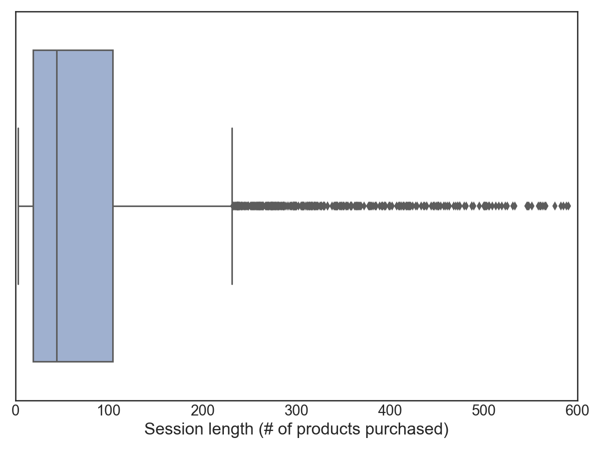
In this case, we define a session as a customer’s full purchase history (all items purchased in each transaction) over the life of the dataset. Below, we show a boxplot of the session lengths (how many items were purchased by each customer). The median customer purchased 44 products over the course of the dataset, while the average customer purchased 96 products.
Another thing to note is the popularity of individual products. Below, we show the log counts of how often each product was purchased. Most products are not very popular and are only purchased a handful of times. On the other hand, a few products are wildly popular and purchased thousands of times.
This dataset has already been preprocessed (e.g., personally identifying information has already been removed.) The only additional preprocessing we performed was to remove entries that did not contain a customer ID number (which is how we define a session).
Setup
In NEP, we consider a user’s history to recommend items for the future—but, when training models for recommendation, all the data is historical. In order to mimic “real life” behavior, we’ll pretend that we only have access to the user’s first n-1 purchased items, and use those to try to predict the nth item purchased.
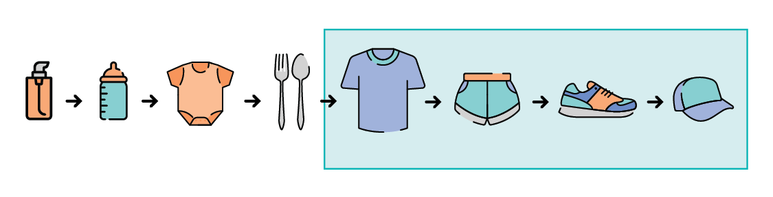
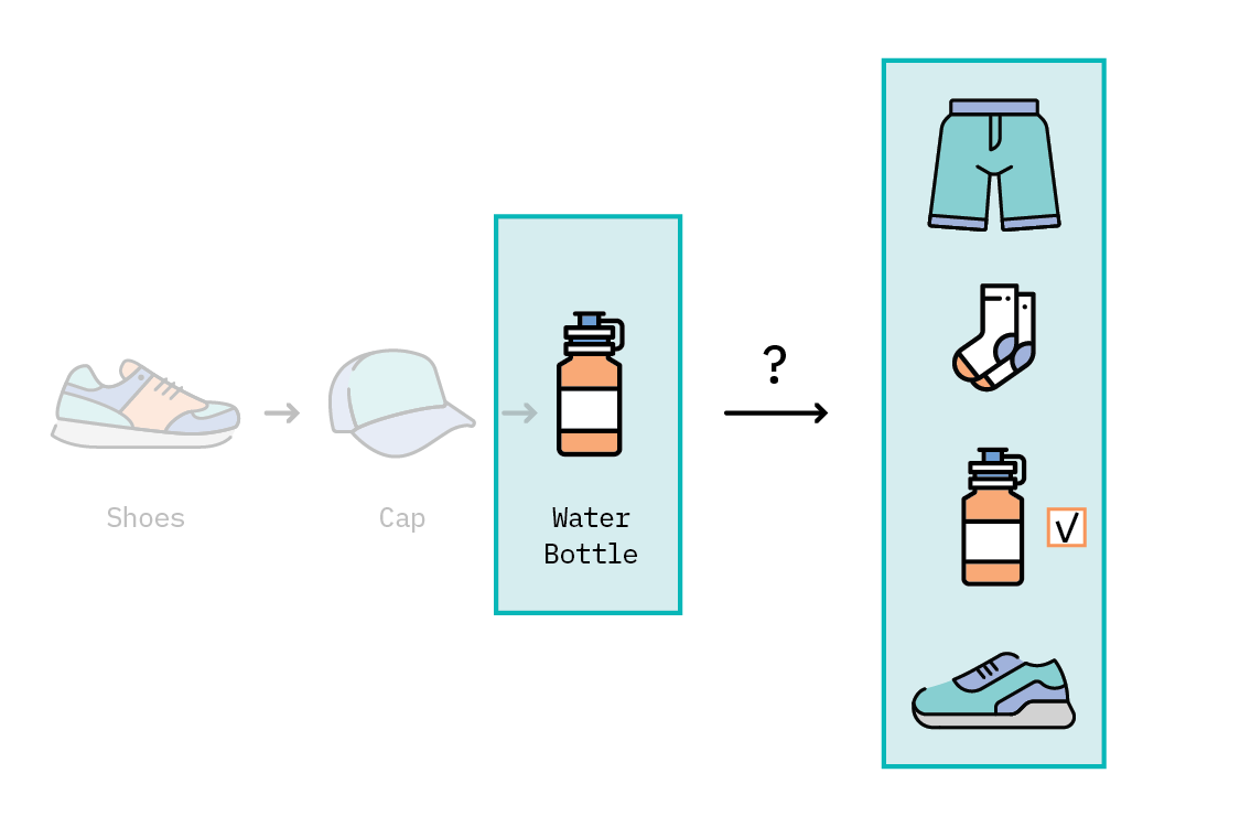
To visualize this, let’s go back to Rhonda’s historical browsing information, collected while she was using our site. We’ll use the highlighted items as our training set to learn product representations, which will be used to generate recommendations. Recommendations are typically based on the most recent interaction by the user, called the query item. In this case, we’ll treat the last item (“cap” in our highlighted set of items below) as the query item, and use that to generate a set of recommendations.
The item outside of the highlighted box (in this case, a “water bottle”) will be the ground truth item, and we’ll then check whether this item is contained within our generated recommendations.
To put it more concretely: for each customer in the Online Retail Data Set, we construct the training set from the first n-1 purchased items. We construct test and validation sets as a series of [query item, ground truth item] pairs. The test and validation sets must be disjoint—that is, each set is composed of pairs with no pairs shared between the two sets (or else we would leak information from our validation into the final test set!).
With this in mind, there is one more preprocessing step that we must apply to our dataset. Namely, we remove sessions that contain fewer than three purchased items. A session with only two, for instance, is just a [query item, ground truth item] pair and does not give us any examples for training.
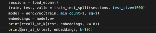
Once we have our train/test/validation sets constructed, it’s time to train! Training Gensim’s word2vec is a one-liner. (For the uninitiated, Gensim is an open-source natural language processing library for training vector embeddings.) We simply pass it the training set and two very important parameters: min_count and sg. min_count is the minimum number of times a word in the vocabulary must be present for word2vec to create an embedding for it. Because we have some rare products, we set this to 1, so that all product IDs in the training set have an embedding. (sg is short for skip-gram, and setting this equal to 1 causes word2vec to use this architecture, as opposed to CBOW.)
Under the hood, word2vec will construct a “vocabulary,” a collection of all unique product IDs, and then learn an embedding for each. Once trained, we can extract the product ID embeddings.
Next, we need to generate recommendations. Given a query item, we’ll generate a handful of recommendations that are the most similar to that item, using cosine similarity. This is the same technique we would use if we wanted to find similar words. Instead of semantic similarity between words, we hope we have learned embeddings that capture the semantic similarity between product IDs that users purchased. Thus, we’ll look for other product IDs that are “most similar” to the query item.
Armed with a list of recommendations, we can now score our model by checking whether the corresponding ground truth item is in our list of recommendations.
We’ll perform this set of operations for each [query item, ground truth item] pair in our test set, to compute an overall score using Recall@K and MRR@K. The output of the code snippet above resulted in a Recall@10 of 19.7 and MRR@10 of 0.108. These results tell us that nearly 20% of the time, the user’s true selection was included in the list of recommendations we generated.
Hyperparameters Matter
In the previous section, we simply trained word2vec using the default hyperparameters-but hyperparameters matter! In addition to the learning rate or the embedding size (hyperparameters likely familiar to many), word2vec has several others which have considerable impact on the resulting embeddings. Let’s see how.
Context window size
The window size controls the size of the context. Recall our earlier example: “The cat jumped over the puddle.” If the context size were set to 6, the entire sentence would be contained within the context window. If we set it to 5, then this sentence would be broken up, and we would instead consider a context like: “The cat jumped over the.” Thus, the context window influences how far apart words can be while still being considered in the same context.
Negative sampling exponent
Word2vec’s training objective is to find word representations that are useful for predicting the surrounding words in the context, by maximizing the average log probability over all possible words.[14] This probability is modeled with the softmax function. Computing the softmax scales with the size of the vocabulary, as such, can become computationally expensive. However, we can approximate the softmax through a technique known as “negative sampling.” In this technique, the model must try to discern between a word that is truly in the context from words that are not part of the context.
Negative samples are chosen from all the other possible words in the corpus based on the frequency distribution of words in that corpus. This frequency distribution is controlled by a hyperparameter called the negative sampling exponent. When this value is 1, common words are more likely to be chosen as negative samples (think stopwords like “the”, “it”, “and”). If the value is 0, then each word is equally likely to be chosen as a negative example (this is a uniform distribution where “the” is just as likely as “cordial”). Finally, if the value is -1, then rare words are more likely to be selected as negative examples.
So, we will train the model to positively identify words belonging to the same context by presenting it with pairs, like [“jumped”, “the”], [“jumped”, “cat”], etc. These are positive examples because “the” and “cat” both appear in the same context as “jumped.” In negative sampling, we will also try to train the model to identify words that are not in the context, by presenting examples like [“jumped”, “airplane”] or [“jumped”, “cordial”]. (These are negative examples because “airplane” and “cordial” are not in the same context as “jumped.”)
Number of negative samples
In addition to the negative sampling exponent, another hyperparameter determines how many negative samples are provided for each positive example. That is, when showing the model [“jumped”, “cat”] (our positive sample), we could include one, five, or maybe even fifty different negative samples.
The code snippet displayed above uses the default values for each of these hyperparameters. These values were found to produce semantically meaningful representations for words in documents, but we are learning embeddings for products in online sessions. The order of products in online sessions will not have the same structure as words in sentences, so we’ll need to consider adjusting word2vec’s hyperparameters to be more appropriate to the task.
| Hyperparameter | Start Value | End Value | Step Size | Configurations |
|---|---|---|---|---|
| Context window size | 1 | 19 | 3 | 7 |
| Negative sampling exponent | -1 | 1 | 0.2 | 11 |
| Number of negative samples | 1 | 19 | 3 | 7 |
| Number of Trials | 539 |
Above, we detail the hyperparameters we considered, the values we allowed these hyperparameters to assume, and the total number of trials necessary to test them all in a sweep. If we want to find the best hyperparameters for our dataset, we’ll need to do quite a bit of training—more than 500 different hyperparameter combinations! We could set up our own code, constructing several nested loops to cover all of the possible parameters—or perhaps we could use sklearn’s GridSearch. However, there’s an even better solution.
Hyperparameter Tuning with Ray
There are several libraries that make hyperparameter optimization approachable, easy, and scalable. For this cycle, we explored Ray.
At its core, Ray is a simple, universal API for building distributed applications. Atop this foundation are a handful of libraries designed to address specific machine learning challenges. Ray Tune provides several desirable features, including distributed hyperparameter sweep, checkpointing, and state-of-the-art hyperparameter search algorithms—all while supporting most major ML frameworks, such as PyTorch, Tensorflow, and Keras.
In our experiments, we tuned over the hyperparameters in the table above for the number of trials specified. Each trial was trained for 100 epochs and was evaluated on the validation set using Recall@10. This resulted in the best hyperparameter configuration for the Online Retail Data Set.
Results
We trained a word2vec model using the best hyperparameters found above, which resulted in a Recall@10 score of 25.18±0.19 on the validation set, and 25.21±.26 for the test set. These scores may not seem immediately impressive, but if we consider that there are more than 3600 different products to recommend, this is far better than random chance!
Hyperparameter Optimization Results
For this dataset, there is actually a wide range of values that would work well for this task. In the following figures, we plot the Recall@10 score for each hyperparameter configuration we tested. Because we tuned over three hyperparameters, we display three figures showing the relationship between pairs of hyperparameters. Essentially, we’ve flattened a 3D space into two dimensions for readability. This means that, for the flattened dimension, we averaged over the Recall@10 scores. For instance, in the left-most figure we plot the number of negative samples against the negative sampling exponent. We average over the Recall@10 scores in the context window dimension, which are the colored points you see in the 2D figure, where yellow indicates a high Recall@10 score and purple is a low score.

In each figure above, the orange star signifies the default word2vec values, and the light blue circle indicates the best hyperparameter configuration we found during our sweep. In all cases, the best hyperparameters are typically in the upper right quadrant; larger values of these hyperparameters perform better than smaller values for this dataset. And in each case, the default word2vec parameters are near, but outside of, the optimal range of values to maximise performance on Recall@10.
We also find two other items of note. First is the size of the context window. In the middle figure, we see that many values of context window size (y axis) will work pretty well, so long as it’s larger than one. (Note that the bottom row of this figure is quite purple, indicating very low relative scores). When the context window is too small, the model is unable to learn relationships between product IDs, and thus recommendations (and our Recall@10 score) suffer. Context matters!
Second is the number of negative samples. In the figure to the far right, we see that more negative samples lead to much better Recall@10 scores. When we select only a single negative example for each positive example, the model again struggles. It is crucial to provide the model with sufficient negative examples. The model must learn not only what things should be in the same context, but especially what things should not be in the same context.
Model Comparisons
Now that we’ve learned the best hyperparameters for our dataset, we can start looking at some model comparisons. We trained models using both our best hyperparameters and the default hyperparameters, each for 100 epochs. The number of epochs is another important parameter, and the default in Gensim’s implementation is five. So we trained another default word2vec model with only five epochs. Finally, we’ve shown the “Association Rules” baseline, a simple heuristic that predicts recommendations based on frequent co-occurrence between items.
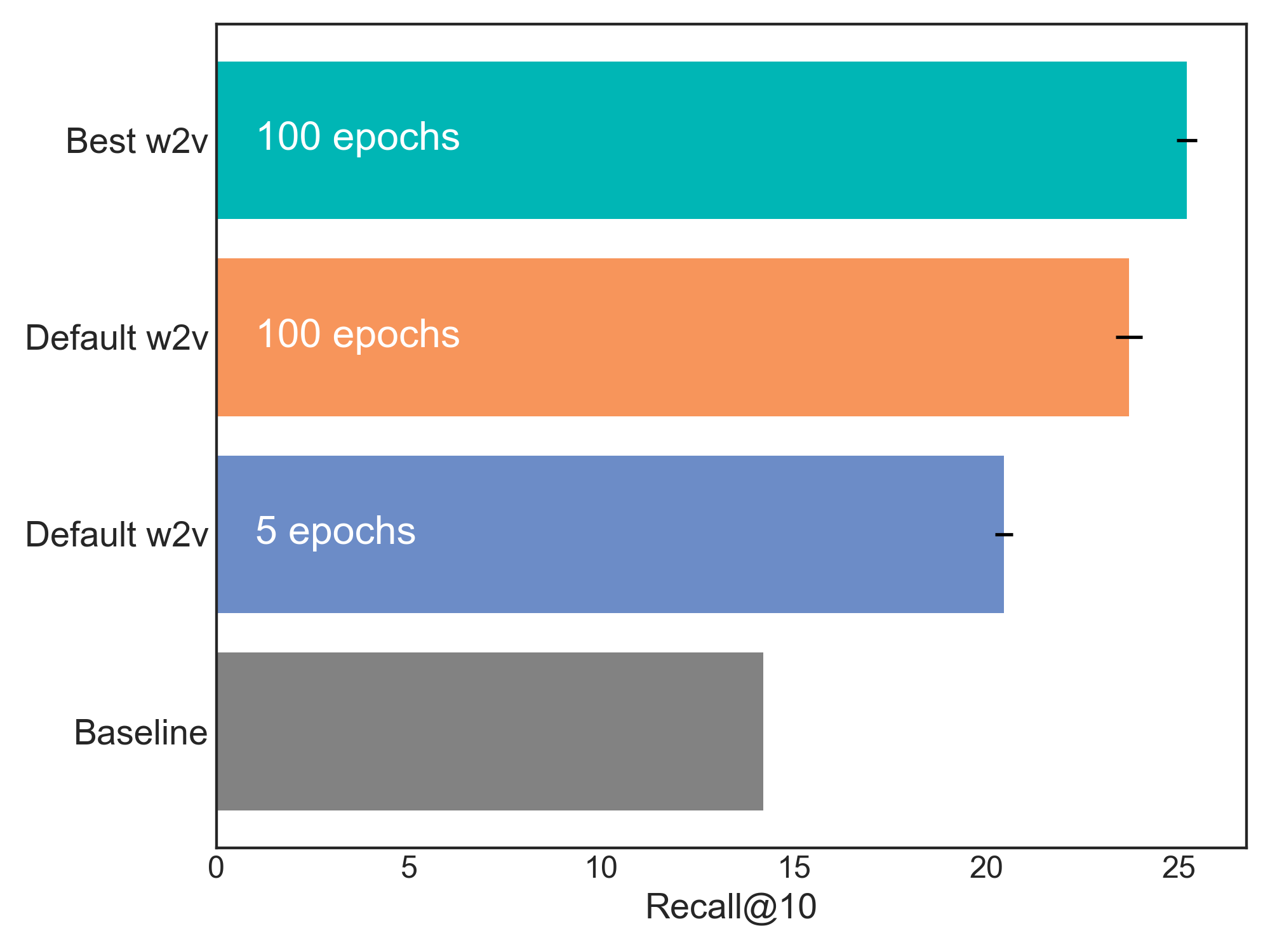
It should be no surprise that the best model is the one configured with the hyperparameters discovered during the tuning sweep—but it turns out the number of training epochs is just as crucial.
We can see the relative contribution of this parameter in Figure 16. The blue bar is the Recall@10 score for a word2vec model trained with all default values, including Gensim’s default of only five epochs of training. The orange bar is the same model trained for 100 epochs. This indicates that simply training word2vec for more epochs can give you a big boost in performance, without doing any hyperparameter sweep at all. But if we train for too many epochs, shouldn’t we be worried about overfitting? Not with word2vec.
With traditional neural networks, we set the number of epochs to minimize the training loss (and increase learning) without overfitting (typically indicated by an increase in the validation loss). However, word2vec is different. We do not care necessarily about the training loss because the goal is to learn embeddings for a downstream task. In this sense, it might not actually matter if the model overfits the training data, so long as the resulting embeddings increase performance on the downstream task, according to whatever metrics we’ve implemented. Therefore, it is almost always beneficial to train word2vec for as many epochs as resources allow, or until the downstream task has reached a performance plateau—in which case, additional training does not yield an increase in the downstream metric.
We can see this effect in the figure below, where we plot word2vec’s training loss in grey and the Recall@10 score on the validation set in blue (since there is no validation loss in this case) as a function of training epochs. The Recall@10 score is completely decoupled from word2vec’s training loss and steadily increases over the course of training. By the end of the 100 epochs, this score has relatively flattened. We tried training for longer (200 epochs), but this didn’t significantly increase performance.
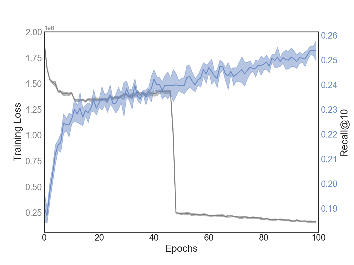
Of course, it’s still better to determine the best set of hyperparameters for the specific dataset you are working with; however, these results demonstrate that you can get far by simply increasing the number of training epochs. We estimate that the increase in training epochs accounts for up to 58% of the performance gains for our best word2vec model (compared to the model trained on default values for only 5 epochs). This suggests that having ideal hyperparameters accounts for roughly 42% of the performance gains, which has performance implications of another kind: computational. Let’s look at some of the challenges of this method for session-based recommendations, starting with the computational cost.
Challenges
While using word2vec to learn product embeddings for recommendations is relatively new and somewhat intuitive, it does come with some challenges. Some of these challenges we faced directly in our experiment, but others are likely to crop up when using this approach for different types of datasets or use cases.
Computational Resources
Using word2vec for product embeddings in a recommendation system can be a viable approach, but for some datasets, identifying the right hyperparameters to optimize those embeddings is a must. The problem is that hyperparameter searches are expensive, requiring one to train hundreds, or even thousands, of model configurations. While the Gensim library[15] is one of the fastest for training vector embeddings, it only supports CPU. GPU support is possible with a Keras wrapper, but benchmarks[16] indicate it is actually slower than the original Gensim CPU version.[17]
However, there are some strategies to mitigate this challenge:
- Perform hyperparameter optimization on a subsample of the original dataset. Although we did not perform this experiment, research[18] has indicated that, for certain datasets, performing hyperparameter optimization on a 10% subsample is sufficient to find good hyperparameters at a fraction of the computational cost.
- Perform a smarter hyperparameter sweep using one of many hyperparameter optimization search algorithms. The idea here is that, overall, fewer trials are needed to find the optimal hyperparameters, thus saving CPU hours.
Metrics
Recall@K and MRR@K are two common metrics for NEP, and provide a way to assess various models on equal footing. However, they don’t directly measure what a business might truly wish to optimize: revenue, watch/listen time, etc.
Recall@K This metric is most practical for settings in which the absolute order does not matter (e.g., the recommendations are not highlighted and they are all shown on the screen at the same time). This might be the case for a website that displays ten or twenty recommendations at once, allowing the user to explore options. However, it’s a harsh metric because it doesn’t assign a score to other items that might be nearly identical to the ground truth item. Recall@K simply assigns a 1 or a 0 depending on whether the user’s true choice was included in the list of recommendations. It does not score any number of similar products in that recommendation list that, in reality, might have been equally acceptable to the user.
MRR@K Mean reciprocal rank is a better choice for applications in which the order of the recommendation matters (e.g., lower ranked recommendations are only shown once the user scrolls to the bottom of the page). In this case, having a higher MRR is crucial, indicating the best recommendations are near the top. Again, this metric only assigns a score if the user’s true choice was included in the list of recommendations and does not give “partial credit” to similar items.
While both of these metrics share similarities with real-world use cases, neither of them directly correlates with increased revenue, watch/listen time, or other real-world KPIs. Furthermore, these metrics do not take into account the quality of the resulting recommendations (more on this in Online evaluation, below). To assess these real-world outcomes, any session-based recommender must be subjected to live, online A/B testing.
The cold start problem
The cold start problem afflicts nearly all recommendation systems, and usually comes in two flavors: new users and new products. For session-based recommendation systems, new users are typically not a problem because these systems do not rely explicitly on user characteristics. As long as a website has some historical user base, that data can be used to generate embeddings for existing products based on how users navigate the site. These embeddings can then generate reasonable recommendations for new users.
However, new products still present a challenge. These items do not have any sessions associated with them in the training dataset; hence, there are no embeddings associated with them, either. A possible solution to this could be to look at a few similar items (for instance, similar products based on domain, or similar music style) and then assign an embedding that is the average of the embedding vectors of the similar items to create an initial vector.
Embeddings and scalability
A general challenge when using word2vec embeddings is that they can be computationally demanding,[19] especially compared to simpler heuristics (such as co-occurrence-based recommendations). Embedding methods require substantial amounts of training data to be effective. Also, in order to actually recommend an item, one needs to compute the closest items (based on cosine similarity, nearest neighbor, or some other distance metric) to a given item using the embeddings. This could be challenging to compute in real time. One way to get around it would be to pre-compute and store the K-closest items to an item for easy lookup when needed. There are also indications that embedding methods[20] may not perform as well as purely sequential models, such as RNNs, although this is likely use-case dependent.
Overall Considerations
The definition of a session is crucial to building a successful session-based recommendation system, but this is not always an easy task. Sessions should be determined based on the structure and type of data collected, as well as the use case or problem at hand. Will the sessions be determined from online browsing history, transactions, rated items, or all of the above? How long should a session be? What determines the session boundary? (For instance, if a user is browsing items on the web, sessions could be delineated based on user inactivity.) All of these questions introduce a number of challenges in designing session-based recommenders. This section summarizes the challenges associated with session-based recommendation systems across various session definitions (length, ordering, anonymous vs. non-anonymous, structure, user actions captured, etc.), as well as the challenges in both determining good recommendations and evaluating them.
Session-related issues
What is more important: a user’s long-term intent or a short-term intent? To this end, we need to consider session lengths while defining the problem. Session lengths can be roughly categorized into three types: long (> 10 interactions), medium (4-9 interactions) and short (<4 interactions). While more interactions could provide more contextual information, they may also introduce noise because they are likely to contain random interactions (due to uncertain user behavior) which are irrelevant to other interactions, leading to poor performance. Similarly, shorter sessions yield only a limited amount of information and, consequently, less context. Based on empirical evidence,[21] medium sessions generally are better at capturing enough contextual information without including too much irrelevant information. This is especially true for transactional data in the ecommerce industry. Selecting an appropriate time span for sessions is domain-dependent, and comes with certain assumptions.
Sessions can also be ordered or unordered, meaning that the user’s interactions may or may not actually capture when the interaction happens. For instance, when shopping online, the order in which a user adds items to their cart may not carry any meaning. Conversely, the sequence of songs listened to may actually matter, reflecting the mood and interests of the user in real time. Such situations warrant looking into appropriate modeling approaches; in some cases co-occurrence-based approaches might work better than sequence models, depending on whether the entries are ordered or unordered.
Another big challenge for session-based recommenders is how to effectively learn from different actions by the user (for instance, how to differentiate between a user’s browsing activity and their purchase activity). Should the session contain only the items that were clicked on? Or should the various actions be combined? If so, how does one model such complex dependencies?
What determines a good recommendation?
Different recommendation strategies and approaches lead to different recommendations. Defining “good” recommendations is challenging because this depends so highly on the use case. For instance, simple baselines use pure co-occurrence between items to generate recommendations, but this might not help a user discover new or lesser known items that might be of interest to them. Additionally, an emphasis on popularity can lead to recommendations that are not diverse.
This is highly relevant in regard to music recommendations. At times, a user may be in the mood to listen to the “most popular” songs, but at other times they are looking to discover something new, in which case popularity-based recommendations are likely not helpful.
Session-based recommenders often tend to make popularity-based recommendations, and this is particularly true of word2vec, which uses co-occurrence within a context to learn item embeddings. These tendencies can be mitigated, in part, by applying popularity or lack-of-diversity penalties to augment the recommendations towards item discovery.[22] Another option could be to include a “popularity metric” for evaluating the recommendations. One could measure an algorithm’s popularity by first normalizing popularity values of each item in the training set, and then, during evaluation, computing the popularity by determining the average popularity value of each item that appears in its top-n recommendation list. (Higher values correspondingly mean that an algorithm has a tendency to recommend rather popular items.)[23]
Online evaluation
Offline evaluations rarely inform us about the quality of recommendations as perceived by the users. In one study of e-commerce session-based recommenders, it was observed that offline evaluation metrics often fall short because they tend to reward an algorithm when they predict the exact item that the user clicked or purchased. In real life, though, there are identical products that could potentially make equally good recommendations. To overcome these limitations, the authors suggest incorporating human feedback on the recommendations from offline evaluations before conducting A/B tests.
Conclusion
Recommender systems have become a cornerstone of online life; they help us navigate an overwhelming amount of information. Being able to predict a user’s interests based on an online session is a highly relevant problem in practice. There is not, however, a one-size-fits-all model; each solution will ultimately be unique to the use case, and care must, as always, be taken in the development and assessment of the model, in order to provide recommendations that will help users and businesses alike. Careful development and assessment of any machine learning model is critical, but it is especially true with recommender systems in general, and session-based recommenders in particular. The best approach is to first benchmark several options on offline metrics (such as Recall@K), and then perform online evaluation (through A/B testing, for instance), before settling on a given model—as offline metrics typically cannot be used to properly assess real-world KPIs (like revenue generation or watch time).
For this report, we experimented with an NLP-based algorithm—word2vec—which is known for learning low-dimensional word representations that are contextual in nature. We applied it to an e-commerce dataset containing historical purchase transactions, to learn the structure induced by both the user’s behavior and the product’s nature to recommend the next item to be purchased. While doing so, we learned that hyperparameter choices are data- and task-dependent, and especially, that they differ from linguistic tasks; what works for language models does not necessarily work for recommendation tasks.
That said, our experiments indicate that in addition to specific parameters (like negative sampling exponent, the number of negative samples, and context window size), the number of training epochs greatly influences model performance. We recommend that word2vec be trained for as many epochs as computational resources allow, or until performance on a downstream recommendation metric has plateaued.
We also realized during our experimentation that performing hyperparameter search over just a handful of parameters can be time consuming and computationally expensive; hence, it could be a bottleneck to developing a real-life recommendation solution (with word2vec). While scaling hyperparameter optimization is possible through tools like Ray Tune, we envision additional research into algorithmic approaches to solve this problem would pave the way in developing more scalable (and less complex) solutions.
Empirical Analysis of Session-Based Recommendation Algorithms ↩︎
Adopted from Applying word2vec to Recommenders and Advertising ↩︎
E-commerce in Your Inbox: Product Recommendations at Scale (PDF) ↩︎
Session-based Recommendations with Recurrent Neural Networks ↩︎
Example taken from Stanford’s popular CS224 NLP lecture series ↩︎
Word2Vec applied to Recommendation: Hyperparameters Matter ↩︎
Distributed Representations of Words and Phrases and their Compositionality ↩︎
One promising lead is the implementation by AWS, BlazingText, which supports multiple CPUs or GPUs. Their benchmarks claim to dramatically decrease training time. ↩︎
Network–Efficient Distributed Word2vec Training System for Large Vocabularies ↩︎
Empirical Analysis of Session-Based Recommendation Algorithms ↩︎